Getting Started with rjuliabugs: A Step-by-Step Logistic Regression Example with Random Effects

This document provides a complete walkthrough for fitting a simple logistic regression model with random effects using the rjuliabugs package. Rather than focusing on deep statistical analysis, the main goal of this guide is to demonstrate how to use the functionality offered by rjuliabugs to fit BUGS models from R by leveraging modern probabilistic programming tools available in Julia.

In particular, rjuliabugs allows users to fit models using advanced samplers such as Hamiltonian Monte Carlo (HMC) and automatic differentiation, as implemented in JuliaBUGS. This integration brings the power and flexibility of modern Bayesian computation into the R ecosystem with full compatibility of well know packages as bayesplot, coda, posterior which provide nice and neat visualizations and diagnosticis for a full Bayesian workflow.

For more technical details about JuliaBUGS, please refer to this link. To learn more about probabilistic programming in Julia, we also recommend the Turing.jl project.

Prerequisites

This vignette assumes that rjuliabugs has already been correctly installed and set up. The goal here is to provide a working example under the assumption that your installation is functional.

For detailed installation instructions and troubleshooting information, please refer to the README. The installation guide includes the following sections:

Data Preparation

To demonstrate a first example, we will use the same dataset presented in the official JuliaBUGS illustration. The case concerns the proportion of seeds that germinated on each of 21 plates. To work with this data, we need to create a named list in R that contains all the variables required by the model.

data <- list(
    r = c(10, 23, 23, 26, 17, 5, 53, 55, 32, 46, 10, 8, 10, 8, 23, 0, 3, 22, 15, 32, 3),
    n = c(39, 62, 81, 51, 39, 6, 74, 72, 51, 79, 13, 16, 30, 28, 45, 4, 12, 41, 30, 51, 7),
    x1 = c(0, 0, 0, 0, 0, 0, 0, 0, 0, 0, 0, 1, 1, 1, 1, 1, 1, 1, 1, 1, 1),
    x2 = c(0, 0, 0, 0, 0, 1, 1, 1, 1, 1, 1, 0, 0, 0, 0, 0, 1, 1, 1, 1, 1),
    N = 21
)

Users already familiar with fitting models using JAGS or Stan will recognize the structure of passing a named list as the data input for the model. Here, we follow the same convention.

One important disclaimer concerns the definition and use of numeric values, particularly integers. When specifying an integer in the data list, make sure it is not written with a decimal point. For example, if a variable like N (e.g., the total number of plates) is defined as 21.0 instead of 21, JuliaCall will automatically convert it as a Float, which may lead to an error if the model expects an Integer. Always use strict integer values when required by the model.

Inspecting closely each element we have r[i] as the number of germinated seeds and n[i] as the total number of seeds on the $i$ -th plate. Let $p_{i}$ be the probability of germination on the $i$ -th plate. Then, the model is defined by:

$\begin{aligned} \text{logit}(p_i) &= \alpha_0 + \alpha_1 x_{1i} + \alpha_2 x_{2i} + \alpha_{12} x_{1i} x_{2i} + b_i \\ b_i &\sim \mathcal{N}(0, \tau) \\ r_i &\sim \text{Binomial}(p_i, n_i) \end{aligned}$

where $x_{1i}$ and $x_{2i}$ are the seed type and root extract of the $i$ -th plate.

BUGS model

Once we have our data prepared, we can define the model using the original BUGS syntax. In rjuliabugs, we write the model as a string in R, following the same structure used in other R packages that interface with BUGS-like tools:

model_def <- "
model {
    for (i in 1:N) {
        r[i] ~ dbin(p[i], n[i])
        b[i] ~ dnorm(0.0, tau)
        logit(p[i]) <- alpha0 + alpha1 * x1[i] + alpha2 * x2[i] +
                       alpha12 * x1[i] * x2[i] + b[i]
    }
    alpha0 ~ dnorm(0.0, 1.0E-6)
    alpha1 ~ dnorm(0.0, 1.0E-6)
    alpha2 ~ dnorm(0.0, 1.0E-6)
    alpha12 ~ dnorm(0.0, 1.0E-6)
    tau ~ dgamma(0.001, 0.001)
    sigma <- 1 / sqrt(tau)
}
"

Users familiar with R packages like R2jags, rjags, or R2WinBUGS will recognize this approach: the model is defined as a string using the BUGS modeling language. For users coming from Stan (e.g., via rstan or cmdstanr), the idea is similar: the model is written as a probabilistic program inside a string object, then compiled and executed by the backend.

This syntactic similarity is not accidental. It is a design choice of rjuliabugs, which aims to allow users to reuse models originally written for JAGS or WinBUGS, while taking advantage of modern features available in Julia—such as Hamiltonian Monte Carlo and automatic differentiation—via JuliaBUGS.

We also remind users that they should be familiar with the BUGS syntax, as syntax-related mistakes will lead to errors during model compilation. For additional guidance, see the Miscellaneous Notes on BUGS from the JuliaBUGS documentation, as well as the BUGS Developer Manual.

For example, writing 1.0E-6.0 instead of 1.0E-6 is a syntax error in BUGS, even though the numerical meaning is equivalent. These types of issues can be subtle but will cause the model to fail during parsing, so attention to detail when writing BUGS code is important.

Inference / Running the Sampler

Once the data is defined and the model is set up, we can run the sampler to perform inference. The setup for the HMC sampler uses Not-U-Turn Sampler (NUTS) with the target acceptance probability $(\delta=0.8)$ for step size adaptation. This is done using the main function, juliaBUGS. For example:


library(rjuliabugs)

posterior <- juliaBUGS(
  data = data,
  model_def = model_def,
  params_to_save = c("alpha0", "alpha1", "alpha2", "alpha12", "sigma"),
  n_iter = 2000,
  n_warmup = 1000,
  n_discard = 1000,
  n_chain = 4,
  use_parallel = FALSE,
  n_thin = 1
)
#> Preparing JuliaBUGS setup... DONE!
#> Initialising AbstractMCMC.sample()... DONE!

This will return the MCMC chains, and a brief inspection can be done through summary function

# Generating the summary of the code
summary(posterior,get_summary = FALSE,get_quantiles = FALSE)
#> Summary of JuliaBUGS sampler:
#> 
#> Iterations        = 3000
#> Number of chains  = 4
#> Number of posterior samples = 2000
#> Thinning parameter = 1
#> Samples per chain = 1001:3000
#> 
#> Summary Statistics:
#> 
#>  parameters      mean     std     mcse ess_bulk ess_tail  rhat ess_per_sec
#>         tau 32.773525 69.4056 3.777707      508    519.7 1.007          NA
#>     alpha12 -0.836158  0.4346 0.007907     3015   3918.0 1.001          NA
#>      alpha2  1.356710  0.2721 0.005125     2785   3940.8 1.003          NA
#>      alpha1  0.083148  0.3190 0.006047     2856   2702.8 1.002          NA
#>      alpha0 -0.551637  0.1947 0.003670     2823   3286.4 1.002          NA
#>        b[1] -0.201474  0.2637 0.005398     2673   3576.3 1.002          NA
#>        b[2]  0.007849  0.2234 0.003023     5612   4172.9 1.002          NA
#>        b[3] -0.204649  0.2312 0.004761     2484   3483.2 1.001          NA
#>        b[4]  0.277397  0.2527 0.005842     1876   4706.6 1.002          NA
#>        b[5]  0.117593  0.2442 0.003727     4573   4427.9 1.001          NA
#>          ...
#>   17 rows omitted

If we wish to obtain the summary statistics for each saved parameter, we can set the argument get_summary = TRUE when calling summary(). Additionally, to include the quantiles associated with the posterior distributions, set get_quantiles = TRUE. To inspect only the summary output in the same format as displayed in JuliaBUGS, set julia_summary_only = TRUE. This will return the native Julia-style summary.

For further details, see the documentation by running ?summary.rjuliabugs.

Inspecting the Posterior Samples

Once sampling is done, the juliaBUGS function returns an object of class rjuliabugs. This object contains:

params
Posterior samples, in the format specified by posterior_type. These are the parameters defined to be saved in the argument params_to_save. The format of this object depends on the prior definition of the argument posterior_type when calling juliaBUGS. The default is "array", which is compatible with most R libraries that work with posterior samples, and returns a 3D numeric array (iterations × chains × parameters). Other available types are "rvar", "mcmc", and "draws". See ?juliaBUGS for more details.
name
Character string identifying the Julia sampler object. As mentioned before, rjuliabugs relies heavily on JuliaCall to integrate the R interface with Julia. While using the package, a Julia session runs in the background and generates the Chains object containing all posterior samples, which can be accessed through the name argument. This name can be defined when calling juliaBUGS through the name parameter and serves as the key to retrieve the fitted sampler. If juliaBUGS is called multiple times with the same name, rjuliabugs automatically generates a new unique name to avoid overwriting. To delete a fitted model object from the Julia environment, call delete_julia_obj() with the corresponding name. See ?delete_julia_obj for more details.
sampler
Sampler object returned by AbstractMCMC.sample. This is a Julia object of type "JuliaObject". For more details, see the documentation of julia_call() in the JuliaCall package.
n_threads
Number of Julia threads detected. This is important to verify whether Julia properly recognized the available threads and if the sampler ran in parallel correctly. If you set parallel = TRUE when calling juliaBUGS but this value is one, the sampler actually ran sequentially.
mcmc
List of MCMC configuration parameters. It includes all MCMC-related arguments passed when calling juliaBUGS.
control
Control options used in the sampler setup. For more details, see the documentation of ?juliaBUGS.

Visualizing Posteriors

Once the posterior samples are obtained, further diagnostic and visualization tools are easily accessible through well-known packages such as bayesplot and posterior. For a full walkthrough of visualizations and diagnostics, check the other vignette (currently in progress).

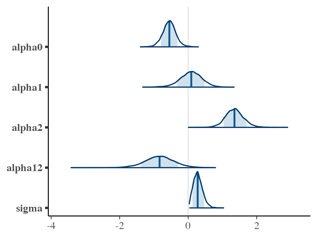
For a quick illustration, let’s observe the density plot of the posteriors and their traceplots.

library(bayesplot)

# Plotting the posterior density for the saved parameters
mcmc_areas(
  posterior$params,
  pars =  c("alpha0", "alpha1", "alpha2", "alpha12", "sigma"),
  prob = 0.8
)

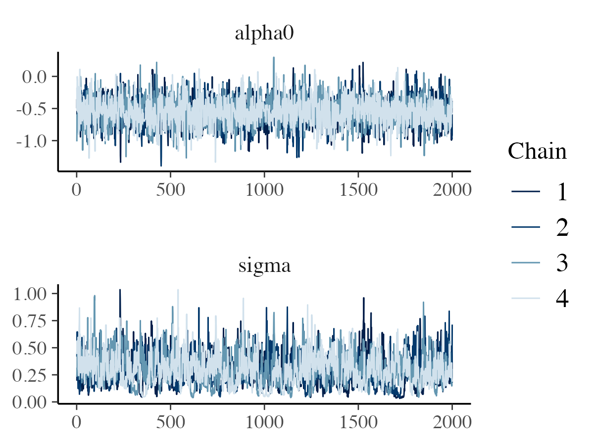
For the traceplots, we subset only the $\alpha_{0}$ and the $\sigma$ parameters:

library(bayesplot)

# Plotting traceplots for alpha0 and sigma
mcmc_trace(
  x = posterior$params,
  pars = c("alpha0", "sigma"),
  n_warmup = 0,
  facet_args = list(nrow = 2)
)

Similarly, diagnostics are also available from the posterior package:

library(posterior)

# For other diagnostics, see the help page
help("diagnostics", "posterior")

# Example: effective sample size
posterior::ess_basic(posterior$params[,,"alpha0"])
#> [1] 2813.332

Saving and loading the `rjuliabugs` model

Lastly, it is important to be able to save and load a rjuliabugs model. To do it so we will use the save_rjuliabugs() to save the posterior object

save_rjuliabugs(rjuliabugs_model = posterior,
                file = "rjuliabugs_model.rds",
                chains_file = "rjuliabugs_chains.jls")

and, to load we use load_rjuliabugs()

posterior <- load_rjuliabugs(file = "rjuliabugs_model.rds")