Plotting rjuliabugs draws using bayesplot package

Overview

This article focuses on plotting parameter estimates from MCMC draws obtained using the rjuliabugs::juliaBUGS() sampler. We do not cover MCMC diagnostics or alternative visualization tools and packages, although these could be easily adapted, since all plots here operate on the params array extracted from the rjuliabugs object. The visualizations shown are based on those presented in the original vignette by Jonah Gabry and Martin Modrák. We strongly recommend reading their article: https://mc-stan.org/bayesplot/articles/visual-mcmc-diagnostics.html. Much of the code and several of the plots here are directly inspired by their examples.

To begin, we load the necessary models to reproduce the examples:

library(bayesplot)
library(ggplot2)
library(rjuliabugs)

Example

As previously mentioned the goal of this vignette is exclusively to show how to use and present some of the visualizations tools from samples obtained from the sampler from rjuliabugs. Therefore we will assume that the rjuliabugs model object is already fitted and named as `rjuliabugs_fit``. For a full walkthrough until this moment, please refer to the article named Get Started until the section where we generate the posterior draws from the sampler

Inspect the params object.

The rjuliabugs is a S3 object which contains all the information and data used in the sampler. This includes, from the the the name of identify the model object in the Julia environment, the mcmc configuration parameters to the posterior draws named as params which by default is given by an 3D numeric array with respective dimensions being (iterations chains parameters). The choice of array as the default is due to its compatibility with most of other packages in R enviroment to work with posterior samplers. However, the converstion to other types to be comptabilite to other packages is possible through the functions as_rvar, as_mcmc and as_draws which can be called over the model object itself (as_rvar(rjuliabugs)) or the rjuliabugs$params object (as_rvar(juliabugs$params). See the reference section for a complete documentation of the examples.

At first we need to extract the posterior samples, to do it so we will use the rjuliabugs::extract function:

pars_names <- c("alpha0","alpha1","alpha2","alpha12","sigma")
posterior_samples <- rjuliabugs::extract(rjuliabugs_fit,pars = pars_names)

Verifying the dimensions of the posterior_samples object we would have

dim(posterior_samples)
#> [1] 2000    4    5

we have a total of 2000 iterations, 4 chains and 5 parameters that were stored.

Posterior uncertainty intervals

Central credible intervals from the posterior distribution can be visualized using the mcmc_intervals function.

mcmc_intervals

color_scheme_set("red")
mcmc_intervals(posterior_samples, pars =  pars_names)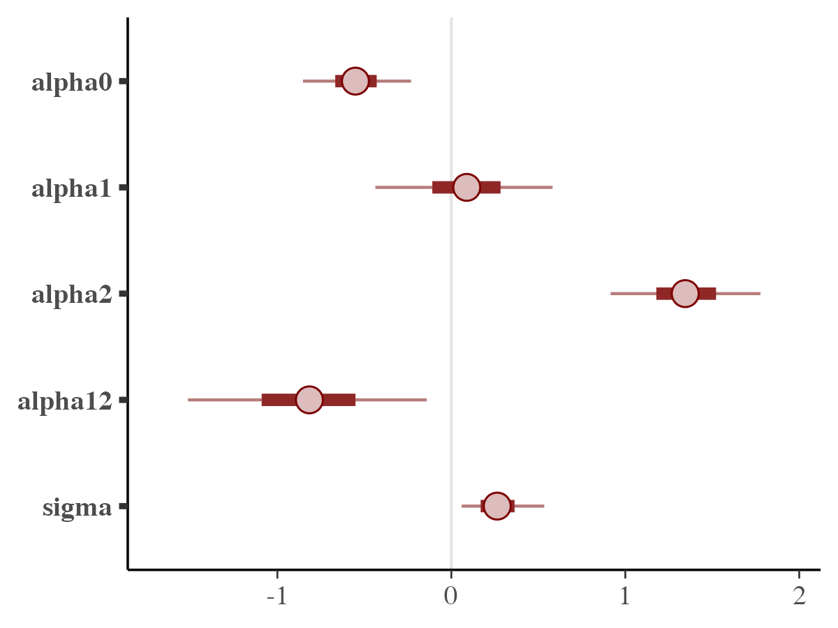

By default, the plot displays 50% credible intervals as bold lines and 90% intervals as thinner outer segments. These settings can be adjusted using the prob and prob_outer parameters, respectively. The plotted points represent the posterior medians; if preferred, the point_est option allows switching to posterior means or suppressing point estimates entirely.

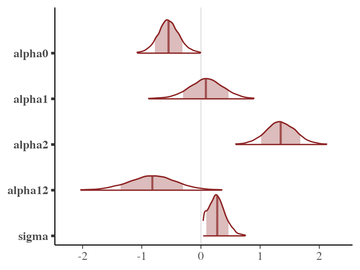
To represent uncertainty with shaded regions beneath the posterior density estimates, the mcmc_areas function can be employed.

mcmc_intervals

mcmc_areas(
  posterior_samples, 
  pars = pars_names,
  prob = 0.8, # 80% intervals
  prob_outer = 0.99, # 99%
  point_est = "mean"
)

mcmc_areas_ridges

We can also generate additional plots with by calling mcmc_areas_ridges

mcmc_areas_ridges(
  posterior_samples, 
  pars = pars_names,
  prob = 0.8, # 80% intervals
  prob_outer = 0.99, # 99%
  point_est = "mean"
)

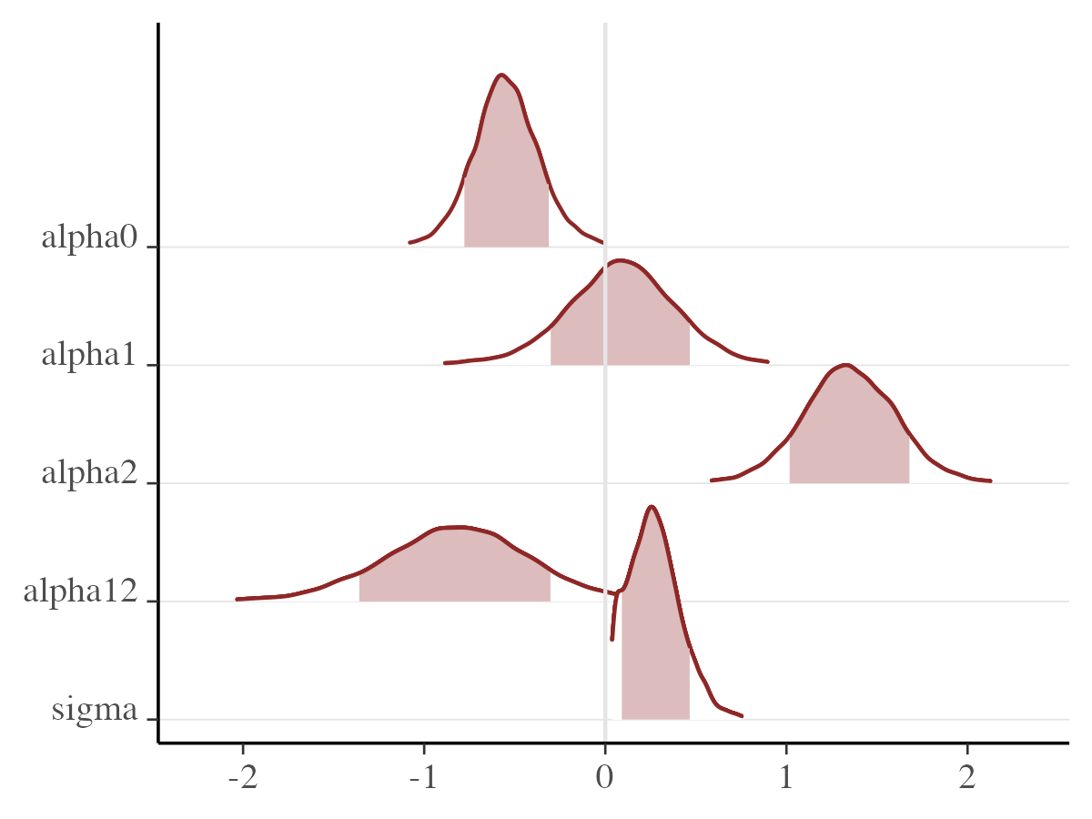## Univariate marginal posterior distributions

The bayesplot package includes functions for visualizing marginal posterior distributions through histograms or kernel density estimates, either by merging all Markov chains or displaying them individually.

mcmc_hist

The mcmc_hist function plots marginal posterior distributions (combining all chains):

color_scheme_set("blue")
mcmc_hist(posterior_samples, pars = c("alpha0", "sigma"))

mcmc_hist_by_chain

To visualize individual histograms for each of the four Markov chains, the mcmc_hist_by_chain function can be used; it generates separate facets for each chain within the plot.

color_scheme_set("darkgreen")
mcmc_hist_by_chain(posterior_samples, pars = c("alpha0", "sigma"))

If we are interested in also display a transformation for display any of the histograms, this is possible by setting the transformations argument.

color_scheme_set("darkgreen")
mcmc_hist_by_chain(posterior_samples, pars = c("alpha0", "sigma"),
                   transformations = list("sigma" = "log"))

Many of the plotting functions for MCMC draws also include a transformations argument to apply transformations to the parameters before plotting.

mcmc_dens

The mcmc_dens function works similarly to mcmc_hist, but it displays kernel density estimates in place of histograms. This include a version of mcmc_dens_by_chain.

color_scheme_set("brightblue")
mcmc_dens(posterior_samples, pars = c("alpha0", "sigma"))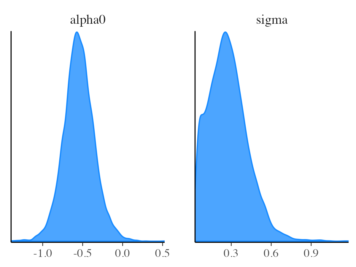

mcmc_dens_overlay

Similar to mcmc_hist_by_chain, the mcmc_dens_overlay function distinguishes between Markov chains; however, rather than showing them in separate panels, it overlays their density estimates in a single plot.

mcmc_dens_overlay(posterior_samples, pars = c("alpha0", "sigma"))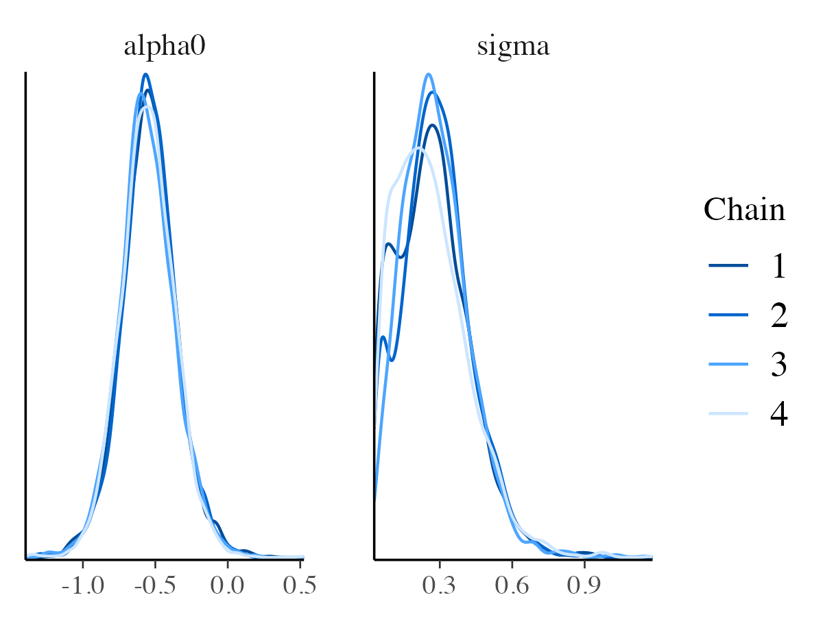

mcmc_violin

The mcmc_violin function visualizes the density estimates for each chain using violin plots and adds horizontal lines at quantiles specified by the user.

color_scheme_set("teal")
mcmc_violin(posterior_samples, pars = c("alpha0", "alpha12"))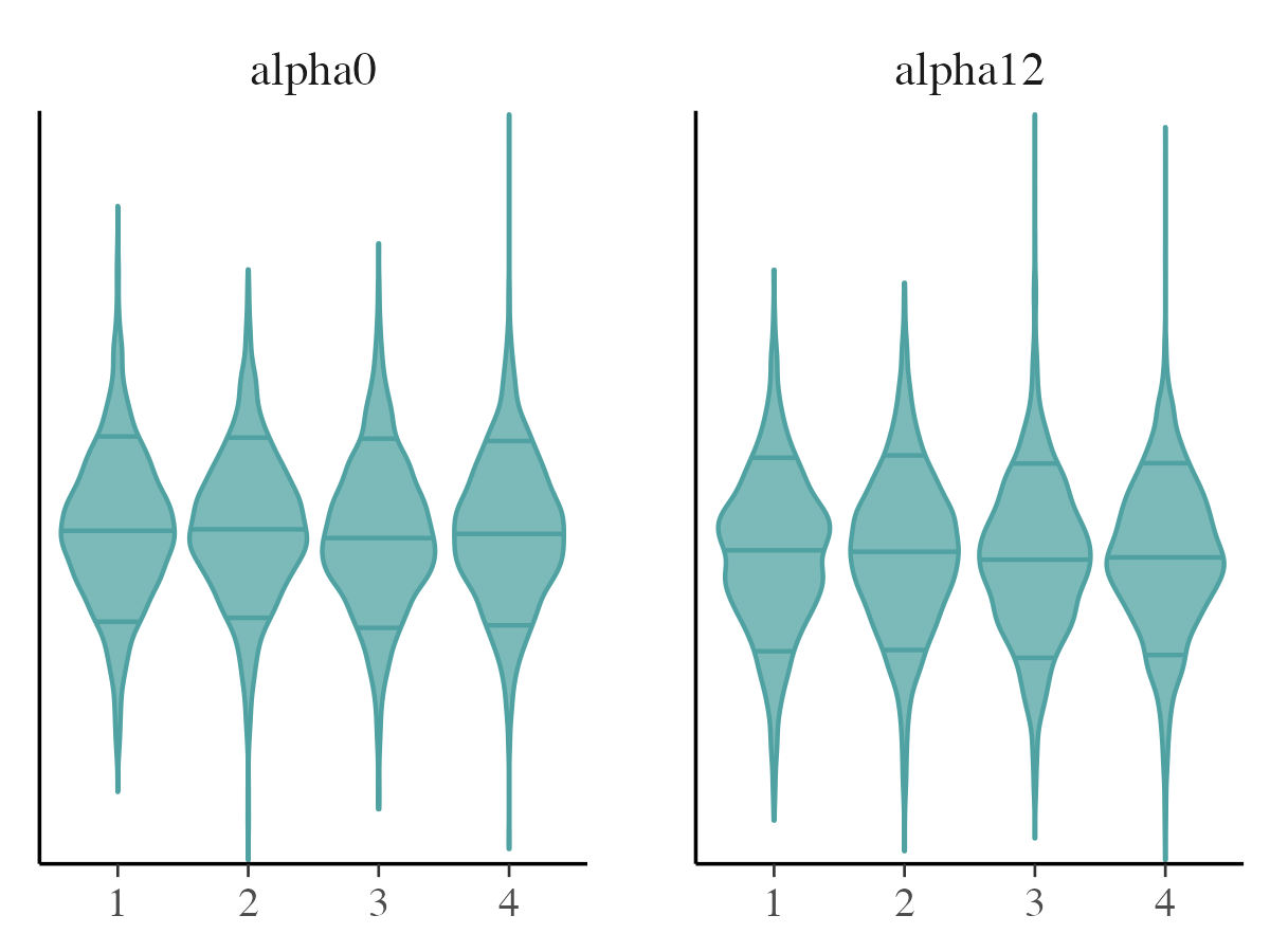

Bivariate plots

A range of functions can be used to visualize bivariate marginal posterior distributions. Several of these functions allow optional parameters to incorporate MCMC diagnostic details into the plots. The extended diagnostic features are explained in a separate vignette focused on visual MCMC diagnostics. The examples here replicate some examples but for complete reference check the original documentation

mcmc_scatter

The mcmc_scatter function generates a basic scatter plot showing the relationship between two parameters.

color_scheme_set("orange")
mcmc_scatter(posterior_samples, 
             pars = c("alpha0", "alpha12"),
             size = 1.5,
             alpha = 0.5)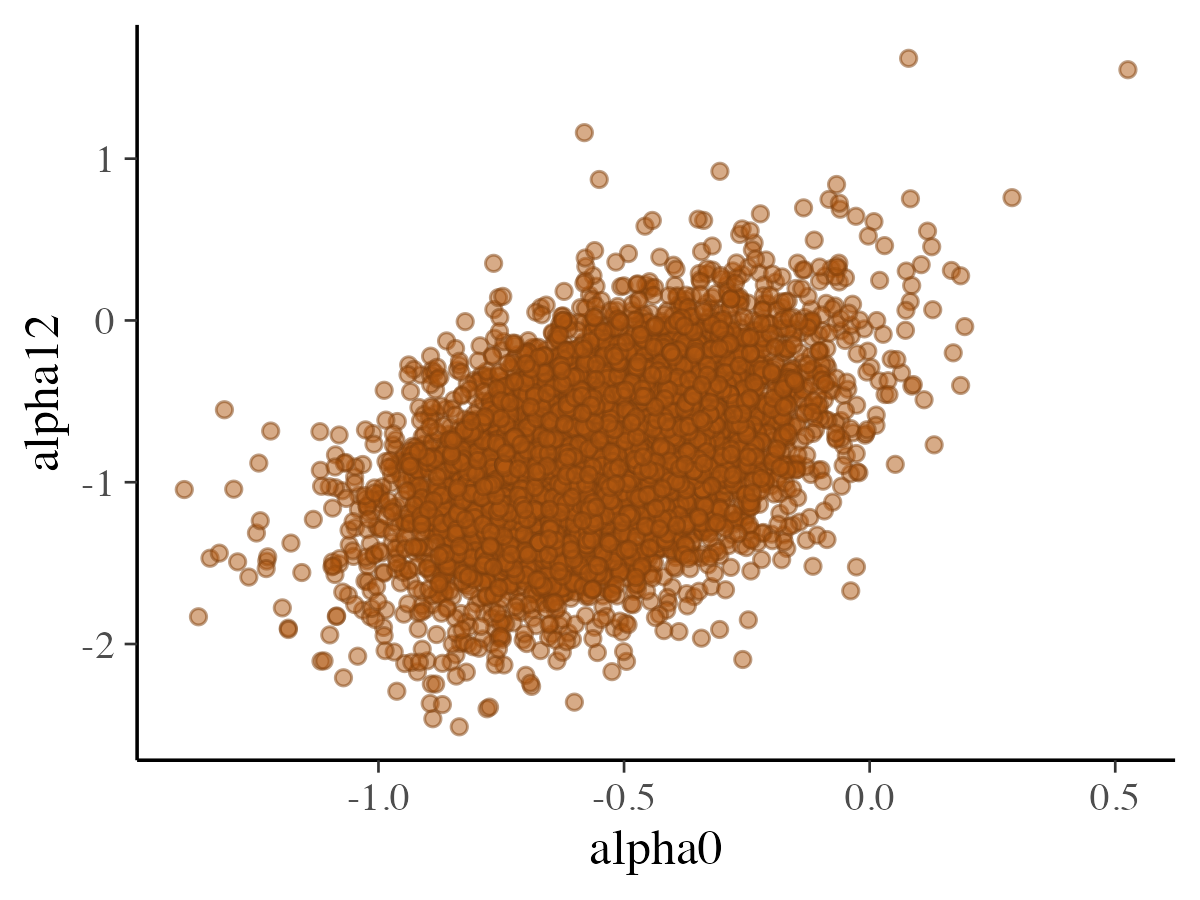

mcmc_hex

The mcmc_hex function produces a comparable plot using hexagonal bins, which helps reduce overplotting when many points overlap.

color_scheme_set("gray")
# requires hexbin package
if (requireNamespace("hexbin", quietly = TRUE)) {
  mcmc_hex(posterior_samples, pars = c("alpha0", "alpha12"))
}

mcmc_pairs

In addition to mcmc_scatter and mcmc_hex, the bayesplot package also includes the mcmc_pairs function, which allows users to create pairs plots for exploring relationships among multiple parameters.

color_scheme_set("purple")
# requires hexbin package
mcmc_pairs(posterior_samples, 
         pars = c("alpha0", "alpha1","alpha12"),
         off_diag_args = list(size = 1.5))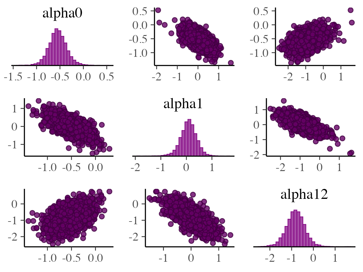

Univariate marginal posterior distributions appear along the diagonal as histograms by default, but this can be switched to density plots using diag_fun = "dens". The bivariate relationships are shown above and below the diagonal using scatter plots, though these can be replaced with hex-bin plots by setting off_diag_fun = "hex". By default, mcmc_pairs splits the Markov chains—showing half above the diagonal and the rest below if the number of chains is even. Additional options for customizing how chains are divided across these plots are available through the condition argument, although these settings are primarily useful when including MCMC diagnostic information. Further details on that are provided in the official vignette from bayesplot documentation named Visual MCMC Diagnostics vignette.

Trace plots

Trace plots display Markov chains smaples, allowing users to inspect how parameter values evolve over iterations. This section presents the standard trace plots available in the bayesplot package.

mcmc_trace

The mcmc_trace function generates basic trace plots to visualize the sampling paths of parameters across iterations.

color_scheme_set("blue")
mcmc_trace(posterior_samples, pars = c("alpha0", "sigma"))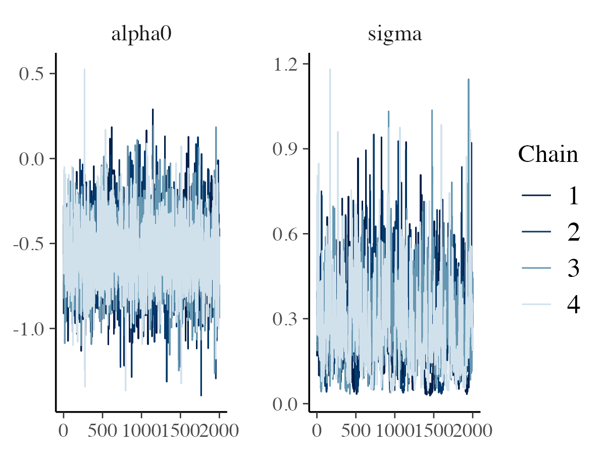

If the differences between chains are difficult to distinguish, a mixed color scheme can be used to improve clarity. For example:

color_scheme_set("mix-blue-red")
mcmc_trace(posterior_samples, pars = c("alpha0", "sigma"),
           facet_args = list(ncol = 1, strip.position = "left"))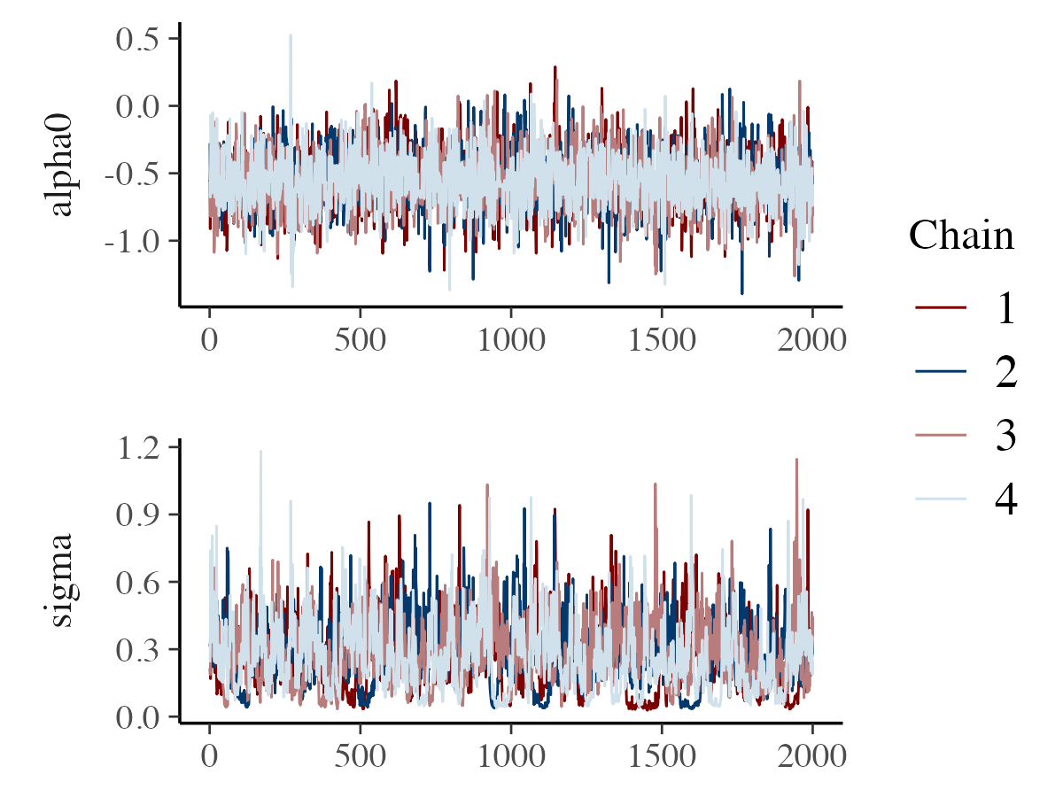

The example above also demonstrates the facet_args argument, which allows you to pass options to ggplot2’s facet_wrap. Setting ncol = 1 stacks the trace plots in a single column, and strip.position = "left" moves the facet labels to the y-axis rather than displaying them above each plot.

mcmc_trace_highlight

The mcmc_trace_highlight function displays points instead of lines and lowers the opacity of all chains except one, which is emphasized using the highlight argument.

color_scheme_set("viridis")
mcmc_trace_highlight(posterior_samples, pars = c( "sigma"),
           highlight = 1)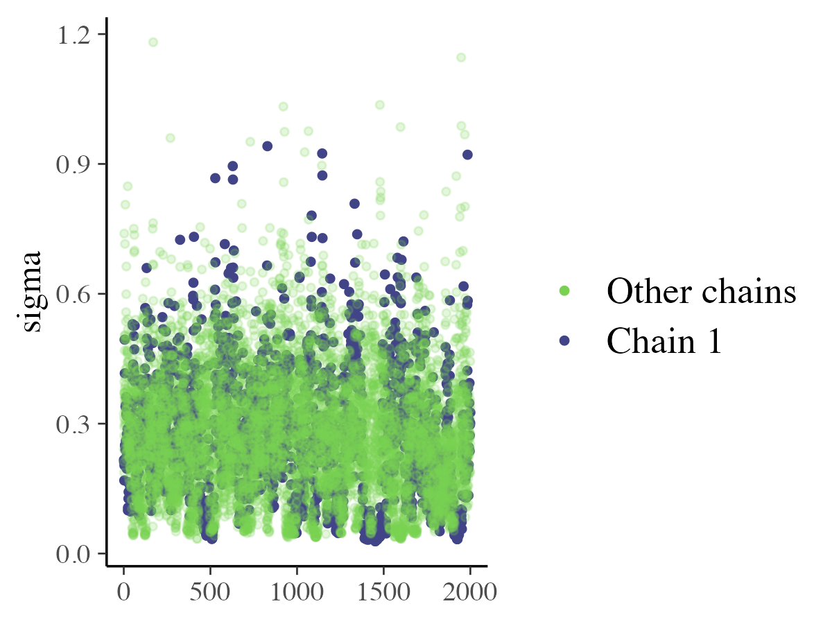

While trace plots focus on how the Markov chains evolve over iterations, mcmc_rank_hist() examines how well the chains mix by comparing the distribution of their ranks. Ideally, the histogram should be roughly uniform, indicating good mixing across chains. See Vehtari et al. (2021) for more background.

mcmc_rank_hist(posterior_samples, pars = c("sigma"))

Additionally, mcmc_rank_ecdf() plots the empirical cumulative distribution functions (ECDFs) of the ranks along with simultaneous confidence bands. These bands have a coverage probability controlled by the prob argument, meaning they are designed to fully contain all rank ECDFs with probability prob. When plot_diff = TRUE, the plot also shows the difference between the observed rank ECDFs and the theoretical uniform distribution expected if all samples came from the same distribution. For more details, see Säilynoja et al. (2022). The function arguments are similar to mcmc_rank_hist.

References

Aki Vehtari, Andrew Gelman, Daniel Simpson, Bob Carpenter, Paul-Christian Bürkner “Rank-Normalization, Folding, and Localization: An Improved R-hat for Assessing Convergence of MCMC (with Discussion),” Bayesian Analysis, Bayesian Anal. 16(2), 667-718, (June 2021)

Säilynoja, T., Bürkner, PC. & Vehtari, A. Graphical test for discrete uniformity and its applications in goodness-of-fit evaluation and multiple sample comparison. Stat Comput 32, 32 (2022). https://doi.org/10.1007/s11222-022-10090-6

Gabry, J., and Goodrich, B. (2017). rstanarm: Bayesian Applied Regression Modeling via Stan. R package version 2.15.3. https://mc-stan.org/rstanarm/, https://CRAN.R-project.org/package=rstanarm

Gabry, J., Simpson, D., Vehtari, A., Betancourt, M. and Gelman, A. (2019), Visualization in Bayesian workflow. J. R. Stat. Soc. A, 182: 389-402. :10.1111/rssa.12378. (journal version, arXiv preprint, code on GitHub)

Gelman, A., Carlin, J. B., Stern, H. S., Dunson, D. B., Vehtari, A., and Rubin, D. B. (2013). Bayesian Data Analysis. Chapman & Hall/CRC Press, London, third edition.

Stan Development Team. (2024). Stan Reference Manual, Version 2.36. https://mc-stan.org

Stan Development Team. (2024). bayesplot: Plotting for MCMC draws. https://mc-stan.org/bayesplot/articles/plotting-mcmc-draws.html